

VCL Web Framework
This is a Node.js application that runs correlation-related experiments of the VCL Lab.
Documentation for the framework is on the git pages here.
Set Up
(1) Git clone the repository
(2) Install Node
Visit the following link to download Node: here.
(3) Install Dependencies
Navigate into the folder:
cd VCLWebFramework
Then run:
npm install
(4) Run the Application
node app.js
Or alternatively, with nodemon:
nodemon app.js
The app is available at localhost:8080. If you want to access it at a different port, change the port number in app.js (line 57).
Terminology
Below is common terminology the lab uses when describing experiments.
Describing an Experiment
Every experiment has the following:
- Experiment : the type of task to be performed.
- Condition : dictated by the task, the method(s) used, and the stimuli type.
- Subcondition : a set of stable constants.
- Trial : marked by the user making a meaningful response/input that is purposely recorded.
- E.g. I am trying to adjust the correlation of a specific plot to be the midpoint between a plot with a high correlation, and a plot with a lower correlation. The final correlation that I have adjusted marks the relevant trial data to be saved.
- Action : the actions a user can make within a trial.
- E.g. In the above trial example, I can be taking actions to increase or decrease my correlation.
Task
The decision task defined in terms of the stimuli and question posed.
- Detection : "there may be any number of alternative stimuli, but one is blank, and the observer is asked only to distinguish between the blank and the other stimuli."
- Discrimination : "there are any number of alternative stimuli, but one of the stimuli (which need not be blank), is designated as the reference, and the observer is asked only to distinguish between the reference and other stimuli."
Method
- Forced Choice : "traditionally characterized by two separate stimulus presentations, one blank and one nonblank, in random order. The two stimuli may be presented successively or side by side. The observer is asked whether the nonblank stimulus was first or second (or on the left or right)."
- Matching : "two stimuli are presented, and the observer is asked to adjust one to match the other."
- Staircase : "for difference thresholds, a variable stimulus is adjusted to increase its absolute difference from a standard stimulus whenever the difference is not discriminated or is adjusted to decrease its absolute difference from the standard stimulus whenever the difference is discriminated."
- E.g. We have two scatter plots side by side. Let us say plot A has r = 0.5 and plot B has r = 0.8. The task is to pick the plot with the higher correlation.
- You correctly pick plot B: So the next trial will be harder, in that the correlations of the two plots are now closer together. For example, plot A would have r = 0.5 and plot B would have r = 0.7.
- You incorrectly pick plot A: So the next trial will be easier, in that the correlations of the two plots are now wider apart. For example, plot A would have r = 0.5 and plot B would have r = 0.9.
- E.g. We have two scatter plots side by side. Let us say plot A has r = 0.5 and plot B has r = 0.8. The task is to pick the plot with the higher correlation.
Properties
- Balancing : the ways in which the subconditions for a given condition are ordered.
- Random
- Latin-Square
- Graph Type : e.g. scatter plots, ring plots, strip plots, shapes
- Graphical Manipulation:
- May be on how the points are plotted e.g. for strip plots, a y coordinate defines the horizontal translation of the "strip" and x coordinate defines the height of the "strip".
- May be in terms of how many distributions are plotted on the same graph e.g. on the same axes, we can have TWO scatter plots with different correlations.
Definitions adapted from:
D. G., & Farell, B. (lOlD). Psychophysical methods. In M. Bass, C. DeCusatis. J. Enoch, V. Lakshmit1arayanan. G. U, C. MacDonald, V. Mahajan & E. V. Stryland (Eds,), Handbook 01 Optics. Third Edition, VDlume III: Visioo and Vision Optics (w. 3.1-3.12). New Yori<: McGraw+liR. http:// psych.nyu,edu/pelilpubslpelIi20 IOpsychophysical-methods,pdt
Condition Identifiers
Each condition is uniquely defined by 4 properties.
Base Experiment
Defines the underlying procedural logic of the experiment.
- JND
- Stevens
- Equalizer
- Estimation
Trial Structure
The trial structure represents the range or pattern of correlation values, and defines a set of constants for each subcondition. Each condition can follow these pattern of values, or use it's own custom structure.
The two main types of patterns are Design or Foundational.
- Foundational : 17 subconditions, base correlation is in the range of [0.0, 0.9] in 0.1 increments.
- Design : 15 subconditions, grouped into five sets with base correlation values set at 0.3, 0.6, 0.9.
- Estimation
- Custom : used when a condition does not follow any of the above structures.
Balancing
How subconditions in a given condition get ordered.
- Randomized
- Latin Square
Graph Types
The type of graph used in the visualization.
- Scatter
- Strip
- Ring
- Shapes
Attributes
Any given condition will always have a base, trial structure, balancing and graph type. However, they will also have a set of variables that manipulate different aspects of the distribution, graphical properties of the visualization, and non-graphical properties such as having a custom instruction set.
Here is a non-comprehensive list of properties that could be manipulated by a condition.
- Experimental attributes:
- Distribution type
- Base correlation of the reference plot
- Whether the correlation converges from above or below
- Complete list of experimental attributes here
- Graphical attributes:
- Some examples if
plot type = scatter:- Point shape
- Point color
- Point size
- Some examples if
plot type = strip:- Line length
- Line width
- Complete list of graphical attributes here
- Some examples if
Architecture
The framework runs on a web-based stack, using JsPsych for experimental logic support and D3 for visualization.
Stack
- Javascript
- Node.js
- Express.js
- JsPsych
- D3.js
- ESDoc (for documentation)
Structure
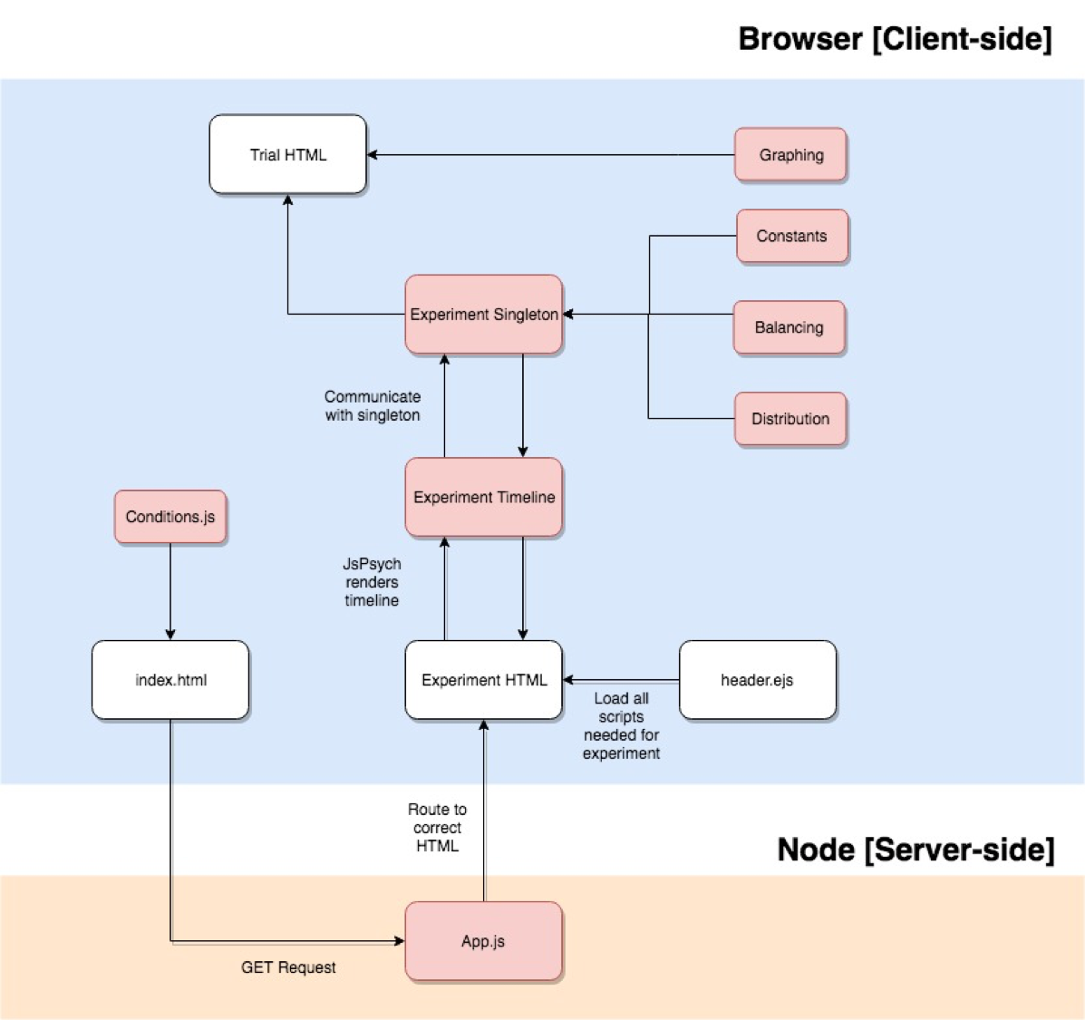
Below is a very high-level overview of the entire structure. Basically:
conditions.jsfeeds into the index to generate the UI, and send the correct identifiers for that condition.- Upon user input on UI, we do a GET request to obtain the correct HTML based on
base experiment. - The experiment HTML is linked to an experiment timeline and model singleton class.
- The timeline uses JsPsych, which helps order the presentation of what is displayed to the user.
- The singleton class extracts the right data, balances subconditions, does any calculations necessary on a trial-by-trial basis, and sends what needs to be presented to the timeline and to the
trial HTML, which displays all trial presentations.
- Experimental properties, such as graphing, constants used, balancing, or the type of distribution, are fed into the singleton or into the trial HTML (since it is doing the displaying).
Experiments
These are the following experiments supported by our framework. The table lists the values for the different identifiers used.
For the Madison's multiple ensemble experiments from December 2018, it is in the repo here - you need to pull the Numerosity-Task and visualSearch branches independently. (So the experiments are NOT on master.)
Look here to understand what identifiers are.
Code Review Process
Below is the process the lab's developers use when reviewing new coded features and conditions to ensure correct functionality and coding standards
Primary Code Reviewers
Below are the people listed as code reviewers for major/critical new features and conditions. Their task is to ensure the code written fits the lab's coding standards and does not introduce new bugs into the framework
- Madison
- Kevin
- Kyle
Peer Code Reviewers
For simpler features and conditions that are not time-sensitive and critical to the functionality of the lab. Peer developers will be done in pairs consisting of a senior and junior lab developer.
Senior Peers
Those who have implemented one or more new conditions or features within the framework
Junior Peers
Those who have just started out in the lab
Stakeholders
Stakeholders are the lab members who requested the new feature/condition. Once the developer is done coding the requested feature/condition, they should confirm with the stakeholder that the code fits their requirements before requesting a code review.
Possible stakeholders are listed below
- Prof. Ronald Rensink
- Madison
- Jessica
- Any researcher at the lab
Code Review Format
Environment
- For non-critical features/conditions, code reviews can be conducted through Google Hangouts and screen shares due to differing schedules
- For critical features relevant to current research, in-person code reviews are recommended
Before the Review
Developers must be able to test the new feature/condition and ensure it's working to stakeholder requirements
For Conditions
- Are all subcondition variable combinations tested?
- Does the data properly save to the csv?
- Are all attributes needed by researchers printed out?
- Did the developer run the esdoc bin update command?
For Features/Changes to Back-End Code
- Does the feature actually work without bugs?
- Were there compromises that were made?
- Is the workflow of the application disrupted in some way?
- Does it do what we want it to do?
The Stakeholder Review
Developers should meet with the stakeholder online/in-person and show the new condition/feature in action. Once the stakeholder gives the approval, the developer can make a pull request and request a code review.
The Code Review Itself
The code review is a meeting between a code-reviewer and a developer. The developer shows the feature in action and the code reviewer and developer look at the actual code to ensure quality.
For the Reviewer:
- Are variables/functions properly named/documented?
- Is there code being repeated? Lots of if cases or functions that seem to do the same thing with only minor differences?
- Are functions too long? If so, make them into helper functions
- Does the new features actually work?
- Potential edge cases?
If additional fixes are needed, the code reviewer must document the requested changes on the created pull request.
Once developer makes additional changes, they must schedule another code review (This one can be shorter or done with image sharing).
Once the code review is complete, the issue can be closed and the pull request merged in.
Practices to Enforce
To ensure consistency and ease of reference for future lab members, it's important to make sure code and documentation follows the same format.
Logistical Practices
Github Issues
This will be primary place to document and assign wanted features/conditions/bugs/experiment types etc ALL requirements, feedback, complications, related issues must be documented in Github Issues
Branch naming
MUST HAVE CONSISTENT NAMING: <issue name>_<developer>
Branch merging
- This requires a pipeline to know which features are ready in the same time frame.
- Group issues together by completion date (Github milestones)
- Constant git pulls. If features take more than a week to implement, must remind them to git pull or rebase from master to update their working copy so they don’t try to merge in outdated code.
Coding Practices
Quick code
- Reduce nested for-loops if possible
- Ensure performance doesn't take a hit
Readable code
- If a function is too bloated move parts into separate helper functions
- If code is repeated across different cases with minimal differences, try combining them into one function
Self-documenting Code
- Variables and functions properly named (no var x = 0;)
- Comments if needed
All new functions need a description in the preamble
- Describe what the function does
- Describe arguments taken in
- Describe in what format the function outputs
- Example input/output if necessary
Documented Mark-Down Files
- Refer to wiki for how-to
- For new experiments or properties
- E.g. since we have new dot types (outlines) these properties need to be documented.
>> JND
- Task: Discrimination
- Method: Forced choice with Staircase
Specifications
_Note that all CAPPED variables are constants taken from the excel sheets/data file._
- For a given subcondition, there are at minimum 24 trials and at maximum 52. Once a user has reached the 24th trial, we start computing for convergence by calculating an F-value to see if it is lower than the threshold.
- If the F-value is <
(1-CONVERGENCE_THRESHOLD), then the current subcondition ends, and proceeds to the next subcondition. - If the F-value is >=
(1-CONVERGENCE_THRESHOLD), then the trials continue.
- If the F-value is <
Practice Procedure
- We choose 4 subconditions randomly, and let the participant run through those. It otherwise follows the same procedure like the test detailed below.
Test Procedure
- For a given subcondition's trial:
- The BASE_CORRELATION for that subcondition will be used to calculate the distribution of one plot, but we need to calculate the adjusted correlation on a trial-by-trial basis.
- At the first presentation of a trial, there is a need to compute the adjusted correlation.
- If converging from above, we calculate it by:
Math.min(MAX_CORRELATION, BASE_CORRELATION + INITIAL_DIFFERENCE) - If converging from below, we calculate it by:
Math.max(MAX_CORRELATION, BASE_CORRELATION - INITIAL_DIFFERENCE)
- If converging from above, we calculate it by:
- If this is NOT the first presentation of a trial, then use the staircase method to calculate the adjusted correlation.
- If converging from above:
- If the previous trial was correct, adjusted correlation =
Math.max(INITIAL_DIFFERENCE, previous adjusted correlation - MAX_STEP_SIZE) - If the previous trial was incorrect, adjusted correlation =
Math.min(MAX_CORRELATION, previous adjusted correlation + MAX_STEP_SIZE * INCORRECT_MULTIPLIER)
- If the previous trial was correct, adjusted correlation =
- If converging from below:
- If the previous trial was correct, adjusted correlation =
Math.min(INITIAL_DIFFERENCE, previous adjusted correlation + MAX_STEP_SIZE) - If the previous trial was incorrect, adjusted correlation =
Math.max(MIN_CORRELATION, previous adjusted correlation - MAX_STEP_SIZE * INCORRECT_MULTIPLIER)
- If the previous trial was correct, adjusted correlation =
- If converging from above:
- Generate a gaussian distribution using the BASE_CORRELATION and adjusted correlation.
- Plot each distribution onto a separate plot, and randomize whether the right/left plots get the base or adjusted correlation. The manner in which the distribution is plotted varies depending on the type of plot. For example:
- For a conventional strip, the x coordinate defines the horizontal translation while the y coordinate determines the height of the "strip".
- For a conventional ring, the x coordinate defines the horizontal translation while the y coordinate determines the radius of the "ring".
- A user can make keyboard inputs with the "z" or "m" keys. "z" corresponds to the left graph, "m" corresponds to the right graph.
- At the first presentation of a trial, there is a need to compute the adjusted correlation.
- The BASE_CORRELATION for that subcondition will be used to calculate the distribution of one plot, but we need to calculate the adjusted correlation on a trial-by-trial basis.
JsPsych Timeline
General Timeline
- Display instructions
- Ready screen
- Display JND practice trials {
    For a given JND experiment, continue to display trials if:
    - There are still more practice subconditions
  }
- Stop screen
- Ready screen
- Display JND test trials {
    For a given JND experiment, continue to display trials if:
    - There are still more test subconditions
  }
- Stop screen with data download options
Trial Logic
Within the trial object, all computations for distributions and constants are performed in the on_start() function. This means that prior to a trial executing, we perform ALL operations detailed in this function. This trial object can be found on line 120 in scripts/experiments/jnd.js.
In general, this is what is executed:
on_start: function(){

  // Retrieve the constants (i.e variables listed in the section below) for the given subcondition index i
  var constants = get_constants_for_subcondition(i);

  // Calculate adjusted correlation
  // (Refer to next section for pseudocode of this function)
  var adjusted_correlation = calculate_adjusted_correlation(constants);

  // Save all relevant constants of this trial to the JsPsych data object
  handle_data_saving(constants);

  var base_coordinates = generate_distribution(constants.BASE_CORRELATION,
                                               constants.ERROR,
                                               constants.NUM_POINTS,
                                               constants.NUM_SD,
                                               constants.MEAN,
                                               constants.SD);

  var adjusted_coordinates = generate_distribution(adjusted_correlation,
                                               constants.ERROR,
                                               constants.NUM_POINTS,
                                               constants.NUM_SD,
                                               constants.MEAN,
                                               constants.SD);

  // Randomize position of the base/adjusted correlations to be either left/right
  // and keep these positions constant for a given subcondition
  var result = randomize_position(base_coordinates, adjusted_coordinates);

  // Set these correlations to the global D3 variables used for plotting
  left_coordinates = result.left;
  right_coordinates = result.right;

}
Adjusted Correlation
Below is the pseudocode for how the adjusted correlation value is generated for a given trial.
var MIN_CORRELATION = 0.0;
var MAX_CORRELATION = 1.0;
var INCORRECT_MULTIPLIER = 3;

function calculate_adjusted_correlation(constants){

   // If first trial, compute solely using constants:
   if (this_is_the_first_trial()){
      var adjusted_correlation = initialize_adjusted_statistic(constants.CONVERGE_FROM_ABOVE,
                                                               constants.BASE_CORRELATION,
                                                               constants.INITIAL_DIFFERENCE);
   }
   // If not first trial, data from previous trial is needed:
   else{
     var last_JND_trial = get_data_from_last_trial();

     var adjusted_correlation = get_next_adjusted_statistic(last_JND_trial.correct,
                                                            constants.CONVERGE_FROM_ABOVE,
                                                            last_JND_trial.adjusted_correlation,
                                                            constants.BASE_CORRELATION,
                                                            constants.MAX_STEP_SIZE);
   }
   return adjusted_correlation;
}

function initialize_adjusted_statistic(converge_from_above, base_correlation, initial_difference){

  var adjusted_correlation;

  if (converge_from_above){
    adjusted_correlation = Math.min(MAX_CORRELATION, base_correlation + initial_difference); }
  else{
    adjusted_correlation = Math.max(MIN_CORRELATION, base_correlation - initial_difference);
  };

  return adjusted_correlation;
}

function get_next_adjusted_statistic(correct, converge_from_above, adjusted_quantity, base_correlation, max_step_size){

  var next_adjusted_statistic;

  var initial_difference = base_correlation;

  if (converge_from_above) {
    if (correct) {
      next_adjusted_statistic = Math.max(initial_difference, adjusted_quantity - max_step_size);
    } else {
      next_adjusted_statistic = Math.min(MAX_CORRELATION, adjusted_quantity + max_step_size
                                * INCORRECT_MULTIPLIER);
    }
  } else {
    if (correct) {
      next_adjusted_statistic = Math.min(initial_difference, adjusted_quantity + max_step_size);
    } else {
      next_adjusted_statistic = Math.max(MIN_CORRELATION, adjusted_quantity - max_step_size
                                * INCORRECT_MULTIPLIER);
    }
  }

  return next_adjusted_statistic;
}
Constants
These are the constants extracted from the input excel sheets. The values of these constants differ for each sub condition.
- BASE_CORRELATION
- ERROR
- MAX_STEP_SIZE
- CONVERGE_FROM_ABOVE
- INITIAL_DIFFERENCE
- NUM_POINTS
- MEAN
- SD
- NUM_SD
>> JND Radius
- Task: Discrimination
- Method: Forced choice with Staircase
Specifications
_Note that all CAPPED variables are constants taken from the excel sheets/data file._
- For a given subcondition, there are at minimum 24 trials and at maximum 52. Once a user has reached the 24th trial, we start computing for convergence by calculating an F-value to see if it is lower than the threshold.
- If the F-value is <
(1-CONVERGENCE_THRESHOLD), then the current subcondition ends, and proceeds to the next subcondition. - If the F-value is >=
(1-CONVERGENCE_THRESHOLD), then the trials continue.
- If the F-value is <
Test Procedure
- For a given subcondition's trial:
- The BASE_RADIUS for that subcondition will be used to calculate the distribution of one plot, but we need to calculate the adjusted radius on a trial-by-trial basis.
- At the first presentation of a trial, there is a need to compute the adjusted radius.
- If converging from above, we calculate it by:
BASE_RADIUS + INITIAL_DIFFERENCE - If converging from below, we calculate it by:
BASE_RADIUS - INITIAL_DIFFERENCE
- If converging from above, we calculate it by:
- If this is NOT the first presentation of a trial, then use the staircase method to calculate the adjusted radius.
- If converging from above:
- If the previous trial was correct, adjusted radius =
previous adjusted radius - 0.002 - If the previous trial was incorrect, adjusted correlation =
previous adjusted radius + 0.006
- If the previous trial was correct, adjusted radius =
- If converging from below:
- If the previous trial was correct, adjusted correlation =
previous adjusted radius + 0.002 - If the previous trial was incorrect, adjusted correlation =
previous adjusted radius - 0.006
- If the previous trial was correct, adjusted correlation =
- If converging from above:
- Generate the shape using the BASE_RADIUS and adjusted radius.
- Plot each shape side by side, and randomize whether the right/left areas get the base or adjusted shapes.
- A user can make keyboard inputs with the "z" or "m" keys. "z" corresponds to the left graph, "m" corresponds to the right graph.
- At the first presentation of a trial, there is a need to compute the adjusted radius.
- The BASE_RADIUS for that subcondition will be used to calculate the distribution of one plot, but we need to calculate the adjusted radius on a trial-by-trial basis.
Constants
These are the constants extracted from the input excel sheets. The values of these constants differ for each sub condition.
- BASE_RADIUS
- CONVERGE_FROM_ABOVE
- INITIAL_DIFFERENCE
>> Stevens
- Task: Discrimination
- Method: Estimation w/ Bisection
Specifications
_Note that all CAPPED variables are constants taken from the excel sheets/data file._
Practice Procedure
- We choose the first 4 subconditions of the data constants (prior to any balancing being done on the subconditions). It otherwise follows the same procedure like the test detailed below.
- Exclusion criteria is calculated during the practice procedure. 2 values are calculated at the end of every subcondition, then stored to be displayed to the researcher who will then determine whether the participant should be excluded or not.
- We calculate standard deviation using the estimated correlations at the end of a trial (e.g. the value when the user hits space bar).
- To calculate anchoring, summate the final estimated correlation values for when the trial started with the LOW_REF for the middle plot, and the values for when the trial started with the HIGH_REF for the middle plot. So there would be 2 values for when the user started on LOW_REF, and 2 values for when the user started on HIGH_REF. Then take the absolute difference between these 2 sums.
anchoring_value = Math.abs(high_ref_trial_sum - low_ref_trial_sum)
- So essentially, there will be 4 sets of anchoring and standard deviation values.
- A subcondition is flagged if the anchoring value > 0.5 or if the standard deviation is > 0.2.
Test Procedure
- A subcondition's structure is "nested" in a sense, in which the user has 4 tries (TRIALS_PER_ROUND) to set the middle graph to be the midpoint between the two other plots.
- For example: let us say a subcondition is defined to have a high correlation (HIGH_REF) of 1.0 and a low correlation (LOW_REF) of 0. These are the R values for the two comparison plots. However, the starting value for the middle plot (the one that participants adjust) will alternate between starting off as the HIGH_REF or LOW_REF.
- Trial 1: middle graph's starting correlation = LOW_REF
- Trial 2: middle graph's starting correlation = HIGH_REF
- Trial 3: middle graph's starting correlation = LOW_REF
- Trial 4: middle graph's starting correlation = HIGH_REF
- A trial is defined as a series of presentations using the HIGH_REF and LOW_REF values, in which the position of the HIGH_REF and LOW_REF distributions are constant (e.g. in Round 1: right graph = HIGH_REF, left graph = LOW_REF). The positioning of whether the left/right plots get which distribution is random across trials, but consistent within a trial. So Round 2 might have the right graph = LOW_REF and left graph = HIGH_REF instead.
- Within a given trial, the user can use the "z" or "m" keys to decrease or increase respectively the correlation of the middle graph. Once the user believes that their middle correlation is a midpoint between the two straddling graphs, they hit spacebar to lock in their answer. So this process happens 4 times, with (a) the middle graph alternating between taking the LOW or HIGH_REF, and (b) the straddling graphs randomizing in position in terms of whether the left or right get the HIGH and LOW_REF correlations.
- To calculate the estimated correlation with respect to the key press (e.g. they want to increase or decrease the correlation), the following formulas apply:
step_size = (HIGH_REF - LOW_REF) / MAX_STEP_INTERVAL- If increasing the correlation,
estimated_correlation = Math.min(HIGH_REF, last trial's estimated correlation + (Math.random() * step_size) - If decreasing the correlation,
estimated_correlation = Math.max(LOW_REF, last trial's estimated correlation - (Math.random() * step_size)- Within a given trial, all the distributions will refresh (e.g. new distributions will be generated using the HIGH_REF, LOW_REF and estimated correlation values) with a refresh rate defined by REGEN_RATE.
- Within a given trial, the user can use the "z" or "m" keys to decrease or increase respectively the correlation of the middle graph. Once the user believes that their middle correlation is a midpoint between the two straddling graphs, they hit spacebar to lock in their answer. So this process happens 4 times, with (a) the middle graph alternating between taking the LOW or HIGH_REF, and (b) the straddling graphs randomizing in position in terms of whether the left or right get the HIGH and LOW_REF correlations.
- For example: let us say a subcondition is defined to have a high correlation (HIGH_REF) of 1.0 and a low correlation (LOW_REF) of 0. These are the R values for the two comparison plots. However, the starting value for the middle plot (the one that participants adjust) will alternate between starting off as the HIGH_REF or LOW_REF.
- Distributions used are gaussian. The manner in which the distribution is plotted varies depending on the type of plot. For example:
- For a conventional strip, the x coordinate defines the horizontal translation while the y coordinate determines the height of the "strip".
- For a conventional ring, the x coordinate defines the horizontal translation while the y coordinate determines the radius of the "ring".
JsPsych Timeline
- Display instructions
- Ready screen
- Display Stevens practice trials {
    For a given Stevens experiment, continue to display trials if:
    - The person has inputted less than the value of TRIALS_PER_ROUND for a given subcondition, or,
    - There are still more subconditions to show, or
    - The person's performance has not passed the exclusion criteria
  }
- Stop screen
- Ready screen
- Display Stevens test trials {
    For a given Stevens experiment, continue to display trials if:
    - The person has inputted less than the value of TRIALS_PER_ROUND for a given subcondition, or,
    - There are still more subconditions to show
  }
- Stop screen with data download options
Trial Logic
Within the trial object, all computations for distributions and constants are performed in the on_start() function. This means that prior to a trial executing, we perform ALL operations detailed in this function. This trial object can be found on line 123 in scripts/experiments/stevens.js.
In general, this is what is executed:
on_start: function(){

  // Retrieve the constants (i.e variables listed in the section below) for the given subcondition index i
  var constants = get_constants_for_subcondition(i);

  // Save all relevant constants of this trial to the JsPsych data object
  handle_data_saving(constants);

  // Update the estimated correlation
  // (Refer to next section for pseudocode of this function)
  var estimated_correlation = update_estimated_correlation(this.trial, constants, last_trial);

  // Generate the gaussian distributions
  var high_coordinates = generate_distribution(constants.HIGH_REF,
                                               constants.ERROR,
                                               constants.NUM_POINTS,
                                               constants.NUM_SD,
                                               constants.MEAN,
                                               constants.SD);

  var high_coordinates = generate_distribution(constants.LOW_REF,
                                               constants.ERROR,
                                               constants.NUM_POINTS,
                                               constants.NUM_SD,
                                               constants.MEAN,
                                               constants.SD);

  var estimated_coordinates = generate_distribution(estimated_correlation,
                                               constants.ERROR,
                                               constants.NUM_POINTS,
                                               constants.NUM_SD,
                                               constants.MEAN,
                                               constants.SD);

  // Randomize position of the low/high correlations to be either left/right
  // and keep these positions constant for a given subcondition
  if (is_last_trial_of_subcondition(i)){
    var result = randomize_position(high_coordinates, low_coordinates);
  }

  // Set these correlations to the global D3 variables used for plotting
  left_coordinates = result.left;
  right_coordinates = result.right;
  middle_coordinates = estimated_coordinates;

}
Estimated Correlation
Below is the pseudocode for how the estimated correlation value is generated for a given trial.
var MAX_STEP_INTERVAL = 10;

function update_estimated_correlation(trial, constants, last_trial){

  var estimated_correlation;

  // If this is the first trial, we need to initialize the middle correlation value
  if (this_is_the_first_trial()){
    estimated_correlation = Math.random() < 0.5 ? constants.LOW_REF : constants.HIGH_REF;
    trial.data.step_size = (constants.HIGH_REF - constants.LOW_REF) / MAX_STEP_INTERVAL;
  }

  // If there was a key press in the last value, we set this current trial's middle correlation value
  // to be based on that input
  else if (last_trial.key_press != null && last_trial.key_press.is_valid_value){
    if (last_trial.key_press == UP_VALUE){
      estimated_correlation = Math.min(constants.HIGH_REF, last_trial.estimated_correlation + (Math.random() *
      last_trial.step_size));
    }
    else if (last_trial.key_press == DOWN_VALUE){
      estimated_correlation = Math.max(constants.LOW_REF, last_trial.estimated_correlation - (Math.random() *
      last_trial.step_size));
    }
  }

  // If there was no input in the last trial
  else {
    estimated_correlation = last_trial.estimated_correlation;
  }

  return estimated_correlation;
}
Constants
These are the constants extracted from the input excel sheets. The values of these constants differ for each sub condition.
- DISTRIBUTION_TYPE
- ROUND_TYPE
- TRIALS_PER_ROUND
- HIGH_REF
- LOW_REF
- ERROR
- NUM_POINTS
- POINT_SIZE
- POINT_COLOR
- BACKGROUND_COLOR
- TEXT_COLOR
- AXIS_COLOR
- REGEN_RATE
- MEAN
- SD
- NUM_SD
>> Estimation
- Task: Discrimination
- Method: Estimation w/ Bisection
Specifications
- This task presents 2 shapes side by side. One shape is the reference shape, while the other is the modifiable shape, in which the user can increase or decrease the size of the shape (by pressing the M or Z keys). The goal is that the user will adjust the size of the modifiable shape so that it is as equal as possible to the reference shape's area.
- Subconditions:
- 3 types of shapes - circle, square, or triangle
- So there are 3 x 3 = 9 different permutations of paired shapes (e.g. circle-circle, circle-square, circle-triangle etc.) - duplicates (3) = 6 permutations
- 3 sizes that the reference shape can start on - 2cm, 4cm or 6 cm
- 2 ways the modifiable shape can "start" on e.g. they can be either smaller or larger in size than the reference shape
- For 2cm reference shape, low = 1.2, high = 3
- For 4cm reference shape, low = 3.1, high = 5.3
- For 6cm reference shape, low = 5.0, high = 6.5
- Total number of subconditions = 6 [permutation of pairs] x 3 [possible reference sizes] = 18 subconditions
- 3 types of shapes - circle, square, or triangle
- Randomize the order of the 18 subconditions.
On a given subcondition:
- The reference and modifiable shape positions can be either left or right (randomized). So before a subcondition starts, there will be text like "Adjust the shape on the left/right so that its size equals that of the other shape."
- For a given subcondition, there are 4 trials. In each trial, the user basically has to make the modifiable shape the same as the reference shape. On a given trial:
- For trials 1 and 3, the modifiable shape's size will start on the low value as specified above (e.g. if 2cm is the reference shape, then modifiable shape's size is 1.2)
- For trials 2 and 4, the modifiable shape's size will start on the high value as specified above.
- The y position of the shapes relative to each other should be slightly jittered (e.g. if have a circle and square, the circle is not completely aligned with the square, so could be a few pixels higher or lower etc.) - the degree of jitter can be randomized.
- The user can press the z [make shape bigger] or m [make shape smaller] keys.
- The step size of the adjustment will be randomized (so not constant).
- They can adjust for an unlimited amount of times.
- Once satisfied, they hit space bar, which then records the size of their modified shape.
- This happens 3 more times (for the same subcondition).
- After the 4 trials for a given subcondition, experiment then moves to the next subcondition.
Summer 2019 Updates
We implemented a series of new estimation conditions to do with measuring area ratios. Tina's pdf spec is here.
- List of new conditions:
- Square, Circle Interference
- Circle Interference
- Multi Square Interference
- Multi Shape Interference
- Multi Fan Interference
- Absolute Area Ratio
- Absolute Area Ratio Bisection (Variant A)
- Absolute Area Ratio Bisection (Variant B)
- Multi Fan Interference (Part B)
- Multi Square Cutout Interference
- Absolute Area Ratio Flicker
- Absolute Area Ratio Bisection (Variant A) Flicker
- Multi Fan Interference (Part B) Flicker
- Multi Square Cutout Interference Flicker
- ** All the flicker conditions are identical to the original condition of the same name, except there is 1000 ms on and 1000 off duration on the ref shapes.
Code Updates
- There are 4 different kinds of configurations:
- Single-single : one shape on ref side and one on mod side (e.g. anything done before the interference conditions)
- Multi-multi : 2 shapes on ref side and 2 shapes on mod side. On mod side, ONE shape is the one getting modified (e.g. Multi Square Interference, Multi Fan Interference etc.)
- Attributes
mod_side_alignmentandref_side_alignmentdefine the types of alignment on mod/ref side, as sometimes alignment is not the same for both. - Attributes
mod_side_shapesandref_side_shapesneed to be defined to tell framework what kinds of shapes are on each side. - Attributes
mod_ratioandref_rationeed to be defined so the framework knows what area ratio needs to be maintained on each side.
- Attributes
- Bisection : the modi shape is in the center, straddled by 2 ref shapes on left and right. Acts similarly to stevens (e.g. Absolute Area Ratio Bisection)
- Attribute
ref_sizenow takes in array of TWO numbers (since there are 2 ref shapes)
- Attribute
- Interference : one shape on ref side and one on mod side - but the shape on the mod side is a compound shape (e.g. Circle, Square Interference) (AKA a triangle is embedded inside a circle, and the whole thing scales with user input)
- All the graphical code previously in model level AKA
estimation.jsnow lives inside the graphing component as a custom script (estimation_plot.js). - All computations for shape properties like size, x_pos, y_pos etc. is done at model level due to complexity.
- New shapes are the fan and cutout-square shapes, otherwise everything else uses Zoe's D3 code.
- Flicker capability is added on reference shapes - can control duration of how long shapes show, and how long shapes don't show. This essentially then loops e.g. if
duration_on= 1000ms andduration_off= 1500ms, flicker will be: show shapes for 1000ms, then off for 1500ms, then on for 1000ms etc. - Initially all the subconditions were programmatically generated as per Zoe's original code. It was becoming tricky to extend because new conditions did not necessarily generate subconditions in the same way, so to make it easier for Tina to customize her values, I refactored
estimation_data.jsto be similar tojnd_data.jswhere every subcondition attribute is defined (so no longer generated programmatically).
Supported Properties
Identifiers
Below are all the supported values for each of the four identifiers.
Base Experiment
Trial Structure
Balancing
Graph Types
Subcondition Attributes
Below are each of the attributes used to define a subcondition. For experimental attributes, some attributes MUST be defined depending on the experiment. Usually, if you are adding a new condition that uses a pre-existing trial structure, the base subconditions from the trial structure already define all these attributes.
Depending on the graph type of the condition, certain graphical attributes can be customized. They will default to a specific value if they are not defined in your new condition.
Experimental Attributes
Graphical Attributes
Conditions
Below is a list of all supported conditions in the framework organized by experiment.
** 1/2/2019 - Madison's Visual Search + Numerosity experiments from December 2018 can be found here.
Developing New Conditions
For Researchers
If you are planning to add a new condition that uses the base experiments already supported, please provide the following information.
To see what identifiers are supported, refer to the page here.
- Condition Name
- High-Level Description of Condition
- Identifiers
- Base Experiment
- Trial Structure
- Balancing
- Graph Type
- Subconditions
- How many subconditions?
- What is changing on each subcondition? List all variables.
- How are each of the variables being changed? List all equations/computations needed if changing on a trial-by-trial basis.
Example
Let us say you want to make a new condition for a JND Design experiment that changes point size on each grouping of the Design trial structure. This is what your information would look like:
- Condition Name: small_point_sizes
- High-Level Description of Condition: Standard JND scatter plot condition, except point sizes vary between 5 - 13 pixels for each 0.3, 0.6, 0.9 base correlation grouping.
- Identifiers
- Base Experiment: JND
- Trial Structure: Design
- Balancing: Latin Square
- Graph Type: Scatter
- Subconditions
- How many subconditions?: 15
- What is changing on each subcondition? List all variables.: Point size
- How are each of the variables being changed on each subcondition? List all equations/computations needed if changing on trial-by-trial basis.: The design trial structure has 5 groupings of the base_correlation = 0.3, 0.6, 0.9, making 15 total subconditions. For each group, point size is different.
- Group 1 point size = 5 px
- Group 2 point size = 7 px
- Group 3 point size = 9 px
- Group 4 point size = 11 px
- Group 5 point size = 13 px
For Developers
(1) Add to config
- Under
public/config/conditions-config, add a new key and javascript object at the bottom. The object should something like below.- Refer here for what is supported on each identifier (experiment, graph type, trial structure, balancing).
name_of_new_condition: {
    experiment: [],
    graph_type: [],
    trial_structure: [],
    balancing: "",
    display_name: "New condition name",
    display_info: {
        description: "",
        researcher: "",
        developer: ""
    }
}
- Check that when you load the UI, your condition is visible with the identifiers specified.
- Note that
experiment,graph_typeandtrial_structurecan take multiple strings (in an array). So you can have the SAME condition name, with the same kind of subcondition-level manipulation, but different underlying base experiment, different graph type, or different trial structure. Good examples of these are the base experiments that run across JND and Stevens.
If we use the example from above, the JS object looks like this:
small_point_sizes: {
    experiment: ["jnd"],
    graph_type: ["scatter"],
    trial_structure: ["design"],
    balancing: "latin_square",
    display_name: "Small Point Sizes",
    display_info: {
        description: "Standard JND scatter plot condition, except point sizes vary between" +
                     "5 - 13 pixels for each 0.3, 0.6, 0.9 base correlation grouping.",
        researcher: "Caitlin Coyiuto",
        developer: "Caitlin Coyiuto"
    }
}
(2) Add subconditions
- Open the right data file for the experiment - they are under
public/scripts/experiment-properties/data/constants.- How the subconditions work is that for a given trial structure, the application MERGES all attributes defined in the
BASEobject with all attributes defined in theCONDITIONSobject. From the example,small_point_sizesis a JND condition using a design trial structure. So the app generates the subconditions forsmall_point_sizesby merging the attributes fromJND_BASE["design"]andJND_CONDITIONS["small_point_sizes"].
- How the subconditions work is that for a given trial structure, the application MERGES all attributes defined in the
- If the trial structure is already supported, you would only need to add all subconditions in a
key: []structure to theCONDITIONSobject.- Add a new key-value pair into the object for
CONDITIONS, with key being thecondition_nameand the value being an array of associative arrays.- Each associative array = one subcondition.
- The keys for each associative array are any of the attributes found here.
- Some notes:
- The number of entries in the array must match the number of entries in the trial structure array. (E.g. if the design trial structure has 15 subconditions/rows, then the new array under
CONDITIONSmust also have 15 rows). - You can OVERRIDE any of the attributes found in the base subconditions. E.g. you can redefine "point_size" in your subcondition if you are changing it on a subcondition-basis.
- The number of entries in the array must match the number of entries in the trial structure array. (E.g. if the design trial structure has 15 subconditions/rows, then the new array under
- Add a new key-value pair into the object for
An example of a new object holding all subconditions should look something like this:
name_of_new_condition:
[
    {attribute1: ___, attribute2: ____}, //first subcondition

    {attribute1: ___, attribute2: ____}, //second subcondition

    {attribute1: ___, attribute2: ____}, //third...

    {attribute1: ___, attribute2: ____},

    .....                                //Number of rows = number of rows or subconditions in trial structure
]
Using the example from above, we are just changing point_size, so we need to define each of the sizes on every subcondition.
Note that the subconditions for a JND Design already has point_size (look at JND_BASE["design"]). By re-defining the point_size
attribute here, you are OVERRIDING the point_size variable in the base. Also note that the number of rows below are equal to the number of rows in JND_BASE["design"].
small_point_sizes:
    [
    {point_size: 5},

    {point_size: 5},

    {point_size: 5},

    {point_size: 7},

    {point_size: 7},

    {point_size: 7},

    {point_size: 9},

    {point_size: 9},

    {point_size: 9},

    {point_size: 11},

    {point_size: 11},

    {point_size: 11},

    {point_size: 13},

    {point_size: 13},

    {point_size: 13},
    ]
Again, depending on your trial structure, the application will merge the constants you define in CONDITIONS with any that are defined in the BASE to get all attributes for the subconditions. So for this example, all the subconditions for small_point_sizes is whatever is listed in the JND_BASE["design"], plus whatever is defined in the CONDITIONS variable.
[
    {distribution_type: "gaussian", base_correlation: 0.3, error: 0.0001, max_step_size: 0.01,
    converge_from_above: true, initial_difference: 0.1, num_points: 100, mean: 0.5, SD: 0.2,
    num_SD: 2.5, point_color: 'BLACK', axis_color: 'BLACK', text_color: 'BLACK',
    feedback_background_color: 'WHITE', background_color: 'WHITE', point_size: 5}, // <-- point_size is now
                                                                                   // overriden (usually for JND
                                                                                   // design, point_size = 6)

    {distribution_type: "gaussian", base_correlation: 0.6, error: 0.0001, max_step_size: 0.01,
    converge_from_above: true, initial_difference: 0.1, num_points: 100, mean: 0.5, SD: 0.2,
    num_SD: 2.5, point_color: 'BLACK', axis_color: 'BLACK', text_color: 'BLACK',
    feedback_background_color: 'WHITE', background_color: 'WHITE', point_size: 5},
    .....
]
(3) Update instructions
Automatically, the application will use the default instructions specified for each experiment in experiments-config.js if no instructions are specified for the condition. For example, for JND:
  jnd : {
    .....
    instructions: {
      default_images: ["scatter_1.png", "scatter_2.png"],
      default_html: `
        <div align = 'center' style='display: block' >
          <p>In this experiment, two graphs will appear side-by-side.
                <br> Indicate which graph is more correlated by pressing the Z or M key.
                <br> Press any key to continue.
                </p>
                <div style='float: left; margin-right: 5vw'>
                  <img style= 'width: 20vw' src='${ADDRESS}/img/instructions/jnd/image1.png'></img>
                  <p class='small'><strong>Press the Z key</strong></p>
                </div>
                <div style='float:right; margin-left: 5vw'>
                  <img style= 'width: 20vw' src='${ADDRESS}/img/instructions/jnd/image2.png'></img>
                  <p class='small'><strong>Press the M key</strong></p>
                </div>
              </div>
            `
    },
    ......
The default images are scatter_1.png and scatter_2.png, which replace image1.png and image2.png.
If you do not want to use the default images or default html, you will need to tack on an additional instructions key to the conditions object in conditions-config.js.
name_of_new_condition: {
  experiment: [],
  graph_type: [],
  trial_structure: [],
  balancing: "",
  display_name: "New condition name",
  display_info: {
    description: "",
    researcher: "",
    developer: ""
  },
  instructions: {
    name_of_experiment: {
      custom_html: ``
      // OR
      custom_images: ['image1.png', 'image2.png' ... ]
    }
  }
}
Inside the instructions object, you must supply either:
- (a)
custom_html, which takes in raw HTML, and will override thedefault_htmlanddefault_imagesinsideexperiments-config.js, OR - (b)
custom_images, which allows you to replace ONLY thedefault_imagesspecified in theexperiments-config.js.- All instruction images are inside
public/img/instructions. Add your images into the corresponding experiment folder. - Make sure that the number of
custom_imagessupplied equals the number ofdefault_imageslisted insideexperiments-config.js. E.g. if the default uses 2, then you need to supply 2 custom images.
- All instruction images are inside
Using the small_point_sizes example:
small_point_sizes: {
  experiment: ["jnd"],
  graph_type: ["scatter"],
  trial_structure: ["design"],
  balancing: "latin_square",
  display_name: "Small Point Sizes",
  display_info: {
    description: "Standard JND scatter plot condition, except point sizes vary between" +
           "5 - 13 pixels for each 0.3, 0.6, 0.9 base correlation grouping.",
    researcher: "Caitlin Coyiuto",
    developer: "Caitlin Coyiuto"
  },
  instructions: {
    jnd: {
      custom_images: ['small_point_1.png', 'small_point_2.png']
    }
  }
}
(4) Update docs
The docs dynamically gets all the condition data specified in the config files. However, it needs to be compiled to be re-updated.
Run this in the command line:
./node_modules/.bin/esdoc
And check that your condition exists in the Conditions tab.
Developing New Properties
Sometimes, new conditions require new properties to be added to the framework. This section goes through how to add new properties for each identifier.
Trial Structures
To add a new trial structure to an existing experiment:
- In
public/config/trial-structure-config.js, add a new key-object pair. Add the relevant doc information like the pre-existing trial structures. - Make sure that the base experiment supports the new structure:
- In
public/config/experiments-config.js, add the name of the new trial structure under thetrial_structurekey for the correct base experiment. Navigate to the right
public/scripts/data/constants/___data.jsfile for the base experiment. Determine how many subconditions the structure will support, and add the new key-array object under the<experiment_name>_BASEobject. For example:const JND_BASE = { .... new_trial_structure: // <-- [ { ... } { ... } etc. ] }When adding the attributes, make sure you add all attributes that the experiment needs to run. Look at the attributes required for each experiment here.
In
public/scripts/data/custom_subcondition_generator.js, add a new key-object pair underCUSTOM_TRIAL_STRUCTURE_CONDITIONS.var CUSTOM_TRIAL_STRUCTURE_CONDITIONS = { foundational : [], ... new_structure: [] // <-- }
Balancing Types
If you want to add a new way to balance subconditions:
- In
public/config/balancing-config.js, add a new key-object pair. Add the relevant doc information like the pre-existing balancing types. - Create a new generator file inside
scripts/experiment-properties/balancing/generators. It should take the length of the dataset array, and return the ordered indices of the subconditions. E.g., if the dataset has 4 subconditions, the random generator will give back [2, 0, 1, 3] AKA randomize the order of the indices. - Make sure the balancing controller supports the new type. In
scripts/experiment-properties/balancing/balancing_controllers.js, import the function from your generator js, then add another case in the switch statement. - Make sure that the base experiment supports the new structure. In
public/config/experiments-config.js, add the name of the new balancing type under thebalancing_typekey for the correct base experiment.
Graph-Related
In terms of graph-related properties, you could either be adding attributes to an already existing graph type, or adding an entire new type of plot or graph type.
Graphical Attributes
This assumes that you are adding to a pre-existing graph type. E.g. if you want to add stroke_width to the scatter graph type.
- In
public/config/graphing-config.jsadd a key-object pair under theattributesof the graph type. Fill in the doc information, and what the default value is. If the attribute only takes in a fixed set of inputs, add a key calledvalid_inputs: [input1, input2 .... ]. - Add d3 code to handle the new attribute. Open the right js file corresponding to the graph type in
public/scripts/graphing/d3-base-plots.
Graph Types
If you want to add a completely new graph type (AKA plot):
- In
public/config/graphing-config.js, add a new key-object pair for the graph type. Add the doc information, and all the attributes that can be manipulatable by subconditions. - In
public/config/experiments-config.js, add the name of the graph type under the experiment that it will support. - In
public/scripts/experiment-properties/graphing/graphing_controller.js:- Add a new switch case in
plot_distributions. - Add a new "prepare" function - it can be modelled after
prepare_scatter_plot, but in the event that you need to pass additional params which are dependent on the trial data, you can add those in yourattributesobject too (look atprepare_shapes_plot). Basically, the prepare function sets up all the data and attributes needed for a single plot, and passes it into the d3 script that will actually generate the plot.
- Add a new switch case in
- Now you need to write the d3 code, which will take in the the
attributesobject created in yourpreparefunction.- Create a new js file named after the graph type inside
d3-base-plots. - Write your d3 code. You will be appending the chart to a div with id =
graph. So you would be doing something like:let chart = d3.select("#graph") .append("svg") ......
- Create a new js file named after the graph type inside
Point/Shape Types
For some conditions, there may be a need to simply add a new kind of point_type (belonging to scatter graph type) or a new type of shape taken inside the shapes array (belonging to shapes graph type).
- In
public/config/graphing-config.js, add the name of the new kind of point or shape type, either under thevalid_inputskey of scatter'spoint_type, or shapes'shapes. - Add the relevant d3 code in the
public/scripts/experiment-properties/graphing/d3-base-plots. - If adding a new
point-type, openscatter_plot.js, and add a switch case with the d3 code inplot_scatter_points. - If adding a new shape type for
shapes, openshape_plot.js, and add a switch case insidecreate_shape_plot. Write the d3 function to handle that case.
Adding Experiments
In the case you are building an entirely new experiment, you will have to do all of the above, plus build the jsPsych timeline and model object to support the timeline. If you haven't read up on JsPsych, I would suggest you do that first, and at least do the reaction time tutorial.
- In
public/config/experiments-config.js, add a new key-object insideEXPERIMENTS. You need to provide thetrial_structure,graph_type,balancing_type,docs, and allattributesthe experiment supports. Refer to the above ^^ instructions if you are adding any new properties for the identifiers. Create the relevant html files that (a) holds the jsPsych timeline, and (b) displays the trials. E.g. look under
public/views/jnd- there is an HTML for jnd_experiment.html and jnd_trial_display.html.- Create a new folder with the same name as your experiment under
public/viewsfor your experiment. - Add an HTML file called
<experiment_name>_experiment.htmland<experiment_name>_trial_display.html. Inside the experiment HTML, you will pass the routing params from the server side. Literally copy and paste below and change all the
<Experiment Name>tags to the new experiment.<!DOCTYPE html> <html> <head> <title>VCL: <Experiment Name> Experiment</title> <%- include('../header'); %> <script type="text/javascript"> // Routing params from EJS: var params = {"trial_structure": "<%= trial_structure %>", "condition": "<%= condition %>", "graph_type": "<%= graph_type %>", "balancing": "<%= balancing %>", "subject_id": "<%= subject_id %>", "subject_initials": "<%= subject_initials %>"}; </script> <script type="module" src="/scripts/experiments/<experiment_name>/<experiment_name>_timeline.js" ></script> </head> <body> </body> </html>Inside the trial display HTML, we need to call the function to plot the graphs. Copy and paste below, and change the
<experiment name>tags.<!DOCTYPE html> <html> <head> <link rel="icon" href="./img/VCL_favicon.png"> <!-- Scripts: --> <!-- D3: --> <script src = "https://d3js.org/d3.v4.min.js"></script> <script src="https://d3js.org/d3-selection-multi.v0.4.min.js"></script> </head> <body> <div align = "center"> <!-- D3 graph goes here: --> <div id="graph"> </div> <script type="module"> import { <experiment_name>_exp } from "/scripts/experiments/<experiment_name>/<experiment_name>_timeline.js"; import { plot_distributions } from "/scripts/experiment-properties/graphing/graphing_controller.js"; plot_distributions(<experiment_name>_exp); </script> </div> </body> </html>
- Create a new folder with the same name as your experiment under
- Add your data for the experiment.
- In
/scripts/data/constantsadd a new js file called<experiment_name>_data.js. - Add all your subcondition data for the trial structure it supports, and any new conditions. Refer here if you're making a new trial structure, and part 2 of here for the new conditions.
- In
/scripts/data/data_controller.js, import yourBASEandCONDITIONSvariables your data js file.- Add the new base experiment to
EXPERIMENT_BASESandEXPERIMENT_CONDITIONS.
- Add the new base experiment to
- In
- Update server-side routing. Open
app.jsunder root, and add anotherelse ifstatement. Make the response render the<experiment_name>_experiment.htmlthat you recently created. - Add the experimental logic. You need to build: (a) the JsPsych timeline, and (b) a model class to support the timeline. You MAY not need a new model class, especially if your experiment is simple enough and doesn't have a lot trial-by-trial dependencies (e.g. look at the visualSearch branch from here). I would suggest using
JND_Radiusas a base, it is the simplest among the experiments.- Add a new folder under
public/scripts/experiments. - Add two js files, (or one if you don't need the model class), called
<experiment_name>.jsand<experiment_name>_timeline.js. - For the timeline, there should be blocks for:
- The welcome page
- Instructions
- Feedback (if any after a trial)
- Experimental trial
- The end page
- For the model class, you need to be able to:
- Retrieve the right data from the /constants folder
- Balance the data
- Make the trial block (e.g.
generate_trialjsPsych object) - Save any variables that the researchers want saved on a trial-by-trial basis
- Determine what is a correct/incorrect response, and change the next trial's presentation (if the experiment demands it)
- Export the data once the experiment ends
- There is no template for the model class, though there are some functions that you can probably re-use from
JND_Radius(akaprepare_experiment), but a lot of the constants are subject to whatever the experiment needs, and thegenerate_trialobject is task-dependent.
- Add a new folder under
Overriding
There are instances where new conditions or plots cannot be supported naturally by the framework. These usually are unconventional instances. A good example are all the conditions prefixed with distractor_<color>_shades. These conditions plot TWO distributions onto a scatter graph, and additionally do not follow any of the supported trial structures. There is therefore a way to NOT USE the base plots (e.g. anything in d3-base-plots) and to not be dependent on any of the trial structures, so you can create your subconditions dynamically instead of declaring them inside /data/constants.
Custom Plots
Assuming that you have a plot that can be categorized under one of the main graph types, but there is some unconventional set-up involved that may likely break or cause the main base plot code to become messy, create a custom d3 script.
For example, the distractor conditions plot two distributions onto a single scatter plot, and also have a very specific way of plotting points to allow equal occlusion between the distributions. Adding this into this functionality into the d3-base-plots/scatter_plot.js will likely make things very messy. So we created a custom D3 script for it instead (d3-custom-plots/distractor_scatter_plot.js).
- Inside
/scripts/experiment-properties/graphing/custom_graphing_controller.js.- Add an if-else clause inside the function
is_custom_plot. Basically should return true for your condition. - Add an if-else clause inside
prepare_custom_plot, and create a new function that sets up the attributes to be sent to your d3 function. - Import that function at the top of this script.
- Add an if-else clause inside the function
- Create the d3 script. Add a new custom plot script inside
/d3-custom-plots. - Lastly, although the d3 code is customized for your condition, the framework still assumes that your condition uses one of the base plots (e.g scatter, strip etc.). If the new plot doesn't fit "naturally" into these types, then you might as well create a new graph type.
Subcondition Generation
There are two instances where you can have custom code for your subconditions: (1) you want to write code that programmatically generates the subconditions instead of writing your data manually inside /data/constants (so this still means you are following a certain trial structure), or (2) you are NOT following any trial structure altogether, so the trial structure is custom.
Inside /scripts/data/custom_subcondition_generator.js:
- For (1): Add your condition name inside
CUSTOM_TRIAL_STRUCTURE_CONDITIONS, undercustomkey. - For (2): Add your condition name inside
CUSTOM_TRIAL_STRUCTURE_CONDITIONS, under the trial structure it follows. - Then:
- Add an if-else inside
get_subconditionsto route it to your custom generator function. - Write the function below to generate the subconditions.
- Add an if-else inside
Updating Documentation
This documentation is generated using ESDoc, which automatically detects and generates documentation for methods, constants, functions etc. in the framework. This is under tabs Reference and Source at the top.
This manual also has custom pages (AKA under tab Home and what is on the left sidebar). These pages are generated using ESDoc's markdown -> HTML conversion feature, but some pages also use javascript to draw from config files in the framework in order to display all conditions, attributes etc.
These sections will describe how these custom pages work, and how to create new pages.
Project Structure of the Docs
- At root level:
docsfolder - this is basically where everything documentation-related goes..esdoc.json- this is the config file for ESDoc. This file must be updated whenever you're adding new pages or new scripts.- There are three plugins:
esdoc-standard-plugin- adding the address of the md file into thefilesarray will let ESDoc convert the md file into html.esdoc-inject-script-plugin- adding the address of any scripts into thescriptsarray will let ESDoc run these scripts across ALL html files.esdoc-inject-style-plugin- adding the address of any style scripts into thestylesarray will make the CSS available across ALL html files.
- There are three plugins:
- Inside
docsfolder:manualfolder - this is where we add any new css, images, pages, or scripts.- You can IGNORE everything else, we are only touching the
manualfolder as everything else is automatically generated by ESDoc.
Dynamic Sections
Some creative hacking was involved to get ESDoc to draw from the data from the config files in the framework. This means that as devs add new conditions, attributes etc. into the config files, the documentation will also get automatically updated.
- The main .md files that draw from
configareconditions.md,experiments.mdandsupported_properties.mdinsidedocs/manual/pages. These files just have the skeleton text (e.g. no tables). - The
docs/manual/scripts/view-controller.jsscript:- Forcibly injects CDN JQuery + Bootstrap (which ESDoc could not do naturally)
- Calls the renderer scripts depending on HTML id tag
- Anything ending in
-renderer.jsinsidedocs/manual/scriptsdraws from theconfigfiles, creates all HTML tables and appends them to the page. - Note that in
.esdoc.json, under theesdoc-inject-script-plugin, we include the config AND renderer scripts so they can be run throughout the docs.
Creating New Pages
- Inside
docs/manual/pagescreate a new markdown file. Write all your content using markdown syntax. - In
.esdoc.json, add the page address into the array offilesunder the object with plugin nameesdoc-standard-plugin. - ESDoc can now convert the markdown file into HTML. Run:
./node_modules/.bin/esdoc.
Updating Pages or Scripts
If you are changing ANY of the content inside docs/manual, or the config files from the framework have been updated, you must run this script so the documentation updates:
./node_modules/.bin/esdoc